3.2 Polynomial behaviour and graphing
The leading term, zeros, and multiplicities of a polynomial control its large-scale shape. A careful sketch combines these features with intercepts and sign information.
3.2.1 End behaviour and local extrema
End behaviour. The behaviour of a function as \(x\to\infty\) and as \(x\to-\infty\).
For a polynomial \(P(x)=a_nx^n+\cdots\), the leading term \(a_nx^n\) determines end behaviour. Even degree gives matching end directions; odd degree gives opposite directions. A positive leading coefficient points upward as \(x\to\infty\), while a negative one points downward. A degree-\(n\) polynomial has at most \(n-1\) local extrema.
Worked Example: Describing cubic end behaviour
For \(P(x)=2x^3-5x^2+x+1\), the leading term is \(2x^3\). Therefore, \(P(x)\to\infty\) as \(x\to\infty\) and \(P(x)\to-\infty\) as \(x\to-\infty\).
Check Your Work
As \(x\to\infty\), \(P(x)\to-\infty\); as \(x\to-\infty\), \(P(x)\to\infty\).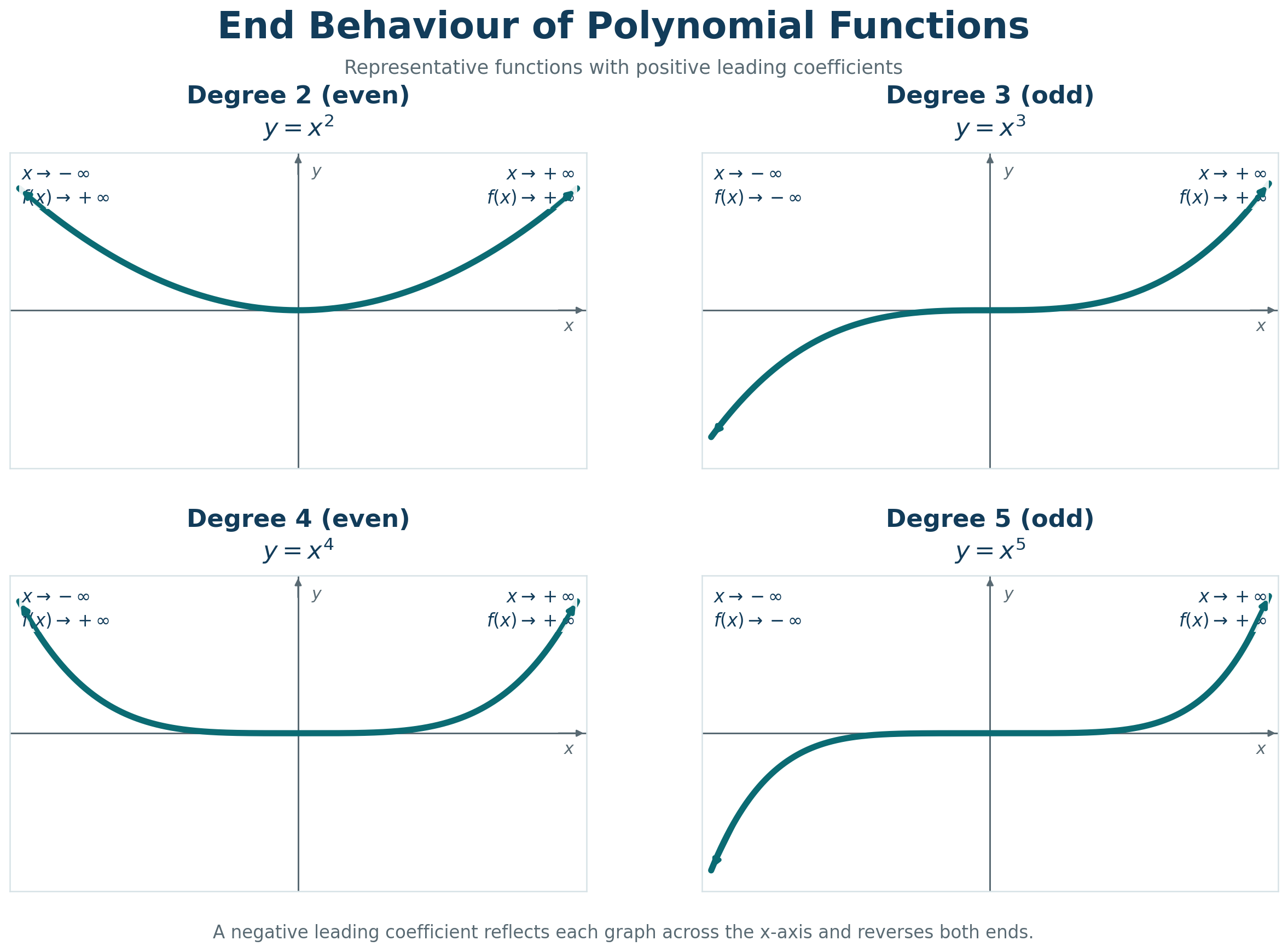
Worked Example: Bounding the number of turns
A fourth-degree polynomial can have at most three local extrema. A graph showing four distinct turning points therefore cannot represent a fourth-degree polynomial.
Check Your Work
Six.3.2.2 Zeros, multiplicity, and a systematic sketch
Multiplicity. The number of times a factor corresponding to a zero occurs in a polynomial.
At a zero of odd multiplicity, a polynomial changes sign and crosses the axis. At a zero of even multiplicity, it touches the axis and turns back. To sketch, factor completely, identify zeros and multiplicities, find the \(y\)-intercept, determine signs between zeros, establish end behaviour, and connect the features smoothly.
Worked Example: Sketching a factored cubic
For \(P(x)=5(x+2)(x-1)(x-3)\), the zeros \(-2\), \(1\), and \(3\) all have multiplicity 1, so the graph crosses at each. The \(y\)-intercept is 30. Positive cubic end behaviour runs from lower left to upper right.
Check Your Work
It crosses at \(x=0\) and touches without crossing at \(x=4\).Worked Example: Interpreting repeated process thresholds
For \(R(q)=-q^2(2q+3)(q-1)\), the zero at \(q=0\) has multiplicity 2, so the graph touches there. It crosses at \(q=-3/2\) and \(q=1\). The negative leading term is degree 4, so both ends point downward.
Check Your Work
It touches at \(x=-1\), crosses at \(x=3\), and has positive odd-degree behaviour from lower left to upper right.Applied Problem: Analyzing a treatment-response polynomial. A dimensionless response is \(R(q)=-0.01q(q-20)^2(q-50)\). Identify the zeros and their multiplicities, state where the graph crosses or touches the axis, and describe its end behaviour.
Check Your Work
The zeros are 0 and 50 with multiplicity 1, and 20 with multiplicity 2. The graph crosses at 0 and 50 and touches at 20. The degree is 4 and the leading coefficient is negative, so both ends approach \(-\infty\).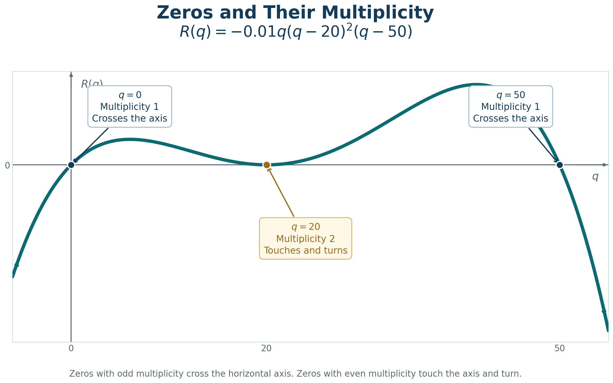
3.2.3 Practice Problems
- Describe the end behaviour of \(3x^4-2x+1\).
Check Your Work
Both ends approach \(\infty\). - Describe the end behaviour of \(-x^3+4x\).
Check Your Work
Left end up, right end down. - State the maximum number of local extrema for degree 6.
Check Your Work
Five. - Identify zeros and multiplicities of \((x+2)^3(x-5)^2\).
Check Your Work
\(-2\) has multiplicity 3; 5 has multiplicity 2. - Find the \(y\)-intercept of \(2(x-1)(x+3)\).
Check Your Work
\(-6\). - A response model is \(P(q)=q(q-10)(q-25)\). At which flows does it cross zero?
Check Your Work
At \(q=0\), 10, and 25. - A model contains \((q-18)^2\). Describe its graph at \(q=18\).
Check Your Work
The zero has even multiplicity, so the graph touches the axis without changing sign. - Describe the end behaviour of the pump polynomial \(-0.2q^4+3q^2\).
Check Your Work
Both ends approach \(-\infty\).