4.1 Exponential functions and transformations
An exponential function places the variable in an exponent. Its constant multiplicative change distinguishes it from a linear function’s constant additive change.
Exponential function. A function \(f(x)=ab^x\), where \(a\ne0\), \(b>0\), and \(b\ne1\).
4.1.1 Basic graphs and properties
For \(f(x)=b^x\), the domain is \(\mathbb R\), the range is \((0,\infty)\), the \(y\)-intercept is \((0,1)\), and \(y=0\) is a horizontal asymptote. The function increases when \(b>1\) and decreases when \(0<b<1\). Equal increases in \(x\) multiply the output by the same factor \(b\).
Worked Example: Identifying an exponential base
An exponential graph passes through \((0,1)\) and \((2,9)\). If \(f(x)=b^x\), then \(b^2=9\). Since an exponential base is positive, \(b=3\) and \(f(x)=3^x\).
Check Your Work
\(b^3=8\), so \(b=2\).Worked Example: Interpreting exponential decay
For \(C(t)=12(0.80)^t\), the initial concentration is \(C(0)=12\). Each time unit multiplies concentration by 0.80, which is a 20% decrease.
Check Your Work
The initial value is 450 and the quantity grows by 6% per time unit.4.1.2 Transformations of exponential graphs
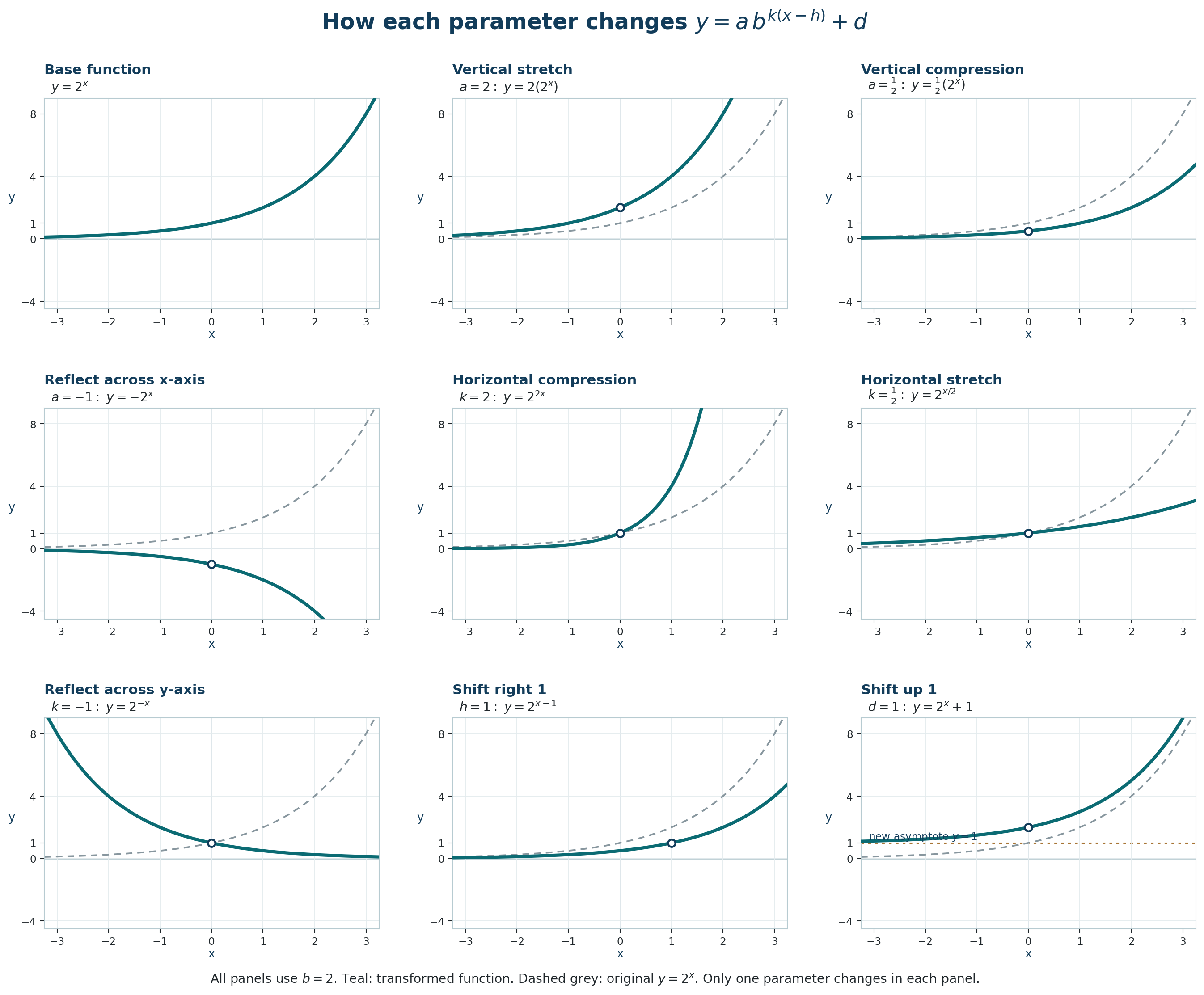
The transformation rules developed in the functions chapter apply. In \(y=ab^{k(x-h)}+d\), \(h\) shifts horizontally, \(d\) shifts vertically, \(a\) changes vertical scale and may reflect the graph, and \(k\) changes horizontal scale. The horizontal asymptote moves from \(y=0\) to \(y=d\).
Worked Example: Transforming an exponential graph
For \(f(x)=2(3^{x-1})+2\), shift \(3^x\) right 1, stretch vertically by 2, and shift up 2. The horizontal asymptote is \(y=2\), and \(f(1)=4\).
Check Your Work
Shift \(2^x\) left 3, reflect across the \(x\)-axis, and shift up 1. The asymptote is \(y=1\).Worked Example: Determining a transformed range
For \(y=5-4(0.5)^x\), the exponential term is positive, so \(y<5\). The domain is \(\mathbb R\), the range is \((-\infty,5)\), and the horizontal asymptote is \(y=5\).
Check Your Work
Range \((-7,\infty)\); asymptote \(y=-7\).Applied Problem: Modelling contaminant decay. A contaminant concentration is initially 18 mg/L and decreases by 15% each day. Write an exponential model, find the concentration after 6 days, and identify the horizontal asymptote.
Check Your Work
\(C(t)=18(0.85)^t\). Then \(C(6)\approx6.79\) mg/L. The horizontal asymptote is \(C=0\).4.1.3 Practice Problems
- State the domain and range of \(4^x\).
Check Your Work
Domain \(\mathbb R\); range \((0,\infty)\). - Does \((1/3)^x\) increase or decrease?
Check Your Work
It decreases because \(0<1/3<1\). - Find the horizontal asymptote of \(2(5^x)-6\).
Check Your Work
\(y=-6\). - Find \(f(3)\) for \(f(x)=7(0.5)^x\).
Check Your Work
\(7/8=0.875\). - Write a model with initial value 80 and growth rate 4%.
Check Your Work
\(f(t)=80(1.04)^t\). - Bacterial concentration begins at 240 cells/mL and grows 8% per hour. Write the model.
Check Your Work
\(N(t)=240(1.08)^t\). - Chlorine concentration begins at 2.4 mg/L and retains 92% each hour. Find it after 5 h.
Check Your Work
\(2.4(0.92)^5\approx1.58\) mg/L. - A transformed treatment model is \(R(t)=60-20(0.7)^t\). State its initial value and limiting value.
Check Your Work
\(R(0)=40\) and the limiting value is 60.