4.2 Exponential models in applications
Exponential models are built from an initial value and a growth factor. Their parameters should be interpreted before calculation so that growth, decay, and units are handled correctly.
4.2.1 Discrete and continuous growth and decay
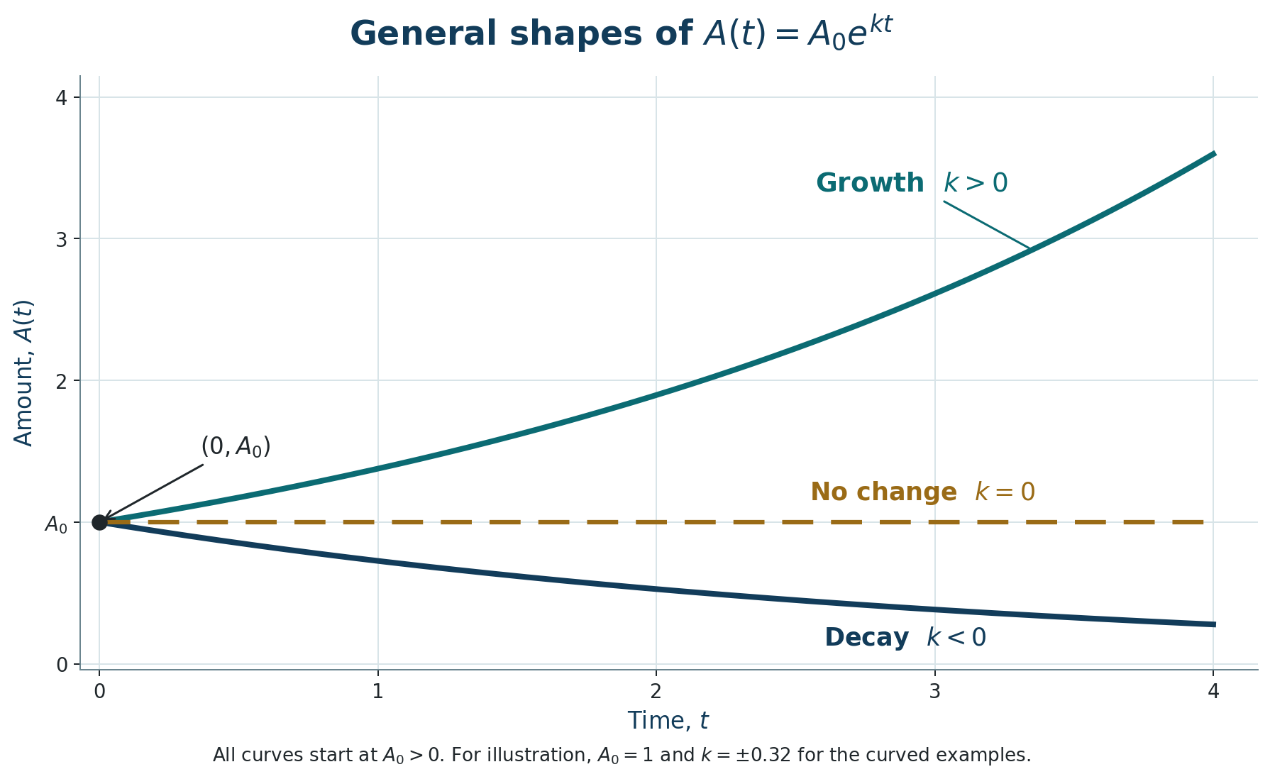
The form \(A(t)=A_0(1+r)^t\) represents a constant proportional change of \(r\) per time period. For decay, \(r\) is negative, or use a factor \(b\) between 0 and 1. Continuous growth or decay uses
\[A(t)=A_0e^{kt},\]
where the sign of \(k\) determines growth or decay.
Compound interest is
\[A(t)=P\left(1+\frac rn\right)^{nt},\]
with principal \(P\), annual rate \(r\), \(n\) compounding periods per year, and time \(t\) in years.
Worked Example: Applying discrete decay
A chemical stock of 50 kg loses 7% per month. After 8 months,
\[A(8)=50(0.93)^8\approx28.0\ \text{kg}.\]
Check Your Work
\(75(1.03)^{10}\approx100.8\).Worked Example: Continuous growth
For \(A(t)=600e^{0.025t}\), the value after 10 years is
\[A(10)=600e^{0.25}\approx770.42.\]
Check Your Work
\(900e^{-0.32}\approx653.53\).4.2.2 Logistic growth
Logistic model. A growth model that approaches a limiting carrying capacity, commonly written \(P(t)=d/(1+ke^{-ct})\) for positive constants \(c\), \(d\), and \(k\).
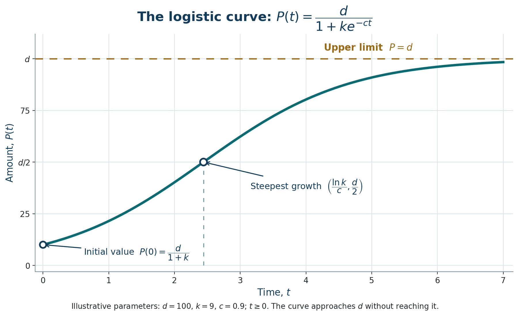
The parameter \(d\) is the long-term limiting population. At \(t=0\), \(P(0)=d/(1+k)\). Logistic growth is initially close to exponential but slows as limited space or resources become important.
Worked Example: Evaluating a logistic model
For \(P(t)=1200/[1+11e^{-0.2t}]\), the initial population is
\[P(0)=\frac{1200}{12}=100.\]
As \(t\to\infty\), the population approaches 1200.
Check Your Work
\(P(0)=800/8=100\) and the limiting value is 800.Worked Example: Comparing two exponential populations
Suppose \(A(t)=1000e^{0.06t}\) and \(B(t)=5000(0.95)^t\). Equality requires
\[1000e^{0.06t}=5000(0.95)^t.\]
Taking logarithms and solving gives \(t=\ln5/[0.06-\ln(0.95)]\approx14.46\) years.
Check Your Work
\(t=\ln2/[\ln(1.04)-\ln(0.98)]\approx11.66\) periods.Applied Problem: Comparing decay models. Chlorine concentration is 3.0 mg/L initially. Model A retains 88% each hour, while Model B follows continuous decay \(C_B(t)=3e^{-0.13t}\). Find both concentrations after 8 h and identify which model predicts the larger residual.
Check Your Work
\(C_A(8)=3(0.88)^8\approx1.08\) mg/L. \(C_B(8)=3e^{-1.04}\approx1.06\) mg/L. Model A predicts the slightly larger residual.4.2.3 Practice Problems
- Identify the initial value and rate in \(A(t)=420(1.05)^t\).
Check Your Work
Initial value 420; growth rate 5%. - Find \(A(6)\) for \(A(t)=1000(0.9)^t\).
Check Your Work
\(531.44\). - Evaluate \(500e^{0.04t}\) at \(t=12\).
Check Your Work
Approximately 808.04. - Find the limit of \(900/[1+5e^{-0.2t}]\) as \(t\to\infty\).
Check Your Work
900. - Find the initial value of \(600/[1+3e^{-0.4t}]\).
Check Your Work
150. - A contaminant retains 81% of its mass each day. What percent is lost daily?
Check Your Work
19%. - A bacterial count of 350 grows continuously at 9% per hour. Find the count after 5 h.
Check Your Work
\(350e^{0.45}\approx549\). - A wetland population follows \(P(t)=2400/[1+5e^{-0.1t}]\). Find its initial and limiting populations.
Check Your Work
Initial 400; limiting 2400.