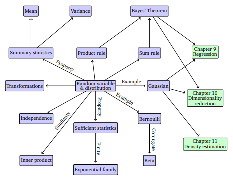
Chapter 6 Probability and Distributions

Probability is the study of uncertainty — it allows us to measure and reason about the likelihood of events. Probability can be interpreted in two complementary ways:

• As the fraction of times an event occurs in repeated experiments.
  
• As a degree of belief in the occurrence of an event.

In machine learning, probability helps us quantify uncertainty in:

• The data we collect,
  
• The models we build, and
  
• The predictions those models make.

Definition 6.1 A random variable is a function that maps outcomes of a random experiment
to numerical or categorical values that we care about.

Formally, the idea of a random variable connects:

• The sample space (possible outcomes),
  
• The events (collections of outcomes),
  
• And the probability distribution, which assigns a likelihood to each outcome or set of outcomes.

Example 6.1 Consider the simple experiment of rolling a fair six-sided die once.

The sample space \(\Omega\) is the set of all possible outcomes: \[ \Omega = \{1, 2, 3, 4, 5, 6\}. \] Each element of \(\Omega\) is a possible outcome of the experiment.

An event is any subset of the sample space. Some examples include:

• Event \(A\): “Roll an even number” \[ A = \{2, 4, 6\}. \]
• Event \(B\): “Roll a number greater than 4” \[ B = \{5, 6\}. \]

A random variable \(X\) is defined as a function: \[ X : \Omega \to \mathbb{R}. \] For example, we could let \[ X(\omega) = \begin{cases} 1, & \text{if } \omega \text{ is even} \\ 0, & \text{if } \omega \text{ is odd} \end{cases}. \] So:

• \(X(2) = 1\), \(X(4) = 1\), \(X(6) = 1\)
  
• \(X(1) = 0\), \(X(3) = 0\), \(X(5) = 0\)

The random variable turns outcomes into numbers.

Since the die is fair, each outcome has probability: \[ P(\{\omega\}) = \frac{1}{6}, \quad \omega \in \Omega. \] The probability distribution of \(X\) assigns probabilities to the values of \(X\): \[ P(X = 1) = P(\{2,4,6\}) = \frac{3}{6} = \frac{1}{2}, \] \[ P(X = 0) = P(\{1,3,5\}) = \frac{3}{6} = \frac{1}{2}. \] Thus, the distribution of \(X\) is: \[ X = \begin{cases} 1 & \text{with probability } \tfrac{1}{2}, \\ 0 & \text{with probability } \tfrac{1}{2}. \end{cases} \]

Big Picture Connection

• Sample space: all possible outcomes (\(\Omega\))
• Events: subsets of outcomes
• Random variable: a function mapping outcomes to numbers
• Probability distribution: probabilities assigned to the values of the random variable.

Definition 6.2 A probability distribution describes how probabilities are spread over the possible values of a random variable.

Probability distributions tell us the chance that specific outcomes will occur. Distributions are foundational tools for:

• Probabilistic modeling,
  
• Graphical models,
  
• Model selection, and
  
• Inference.

Definition 6.3 A probability space consists of three key elements:

1. Sample space – the set of all possible outcomes
   
2. Events – subsets of the sample space
   
3. Probability function – assigns a number between 0 and 1 to each event

These components work together to define how probability is assigned and interpreted.

---