2.0 Vectors
Definition 2.1 A vector is a mathematical object that can be added to other vectors and multiplied by scalars, resulting in another vector of the same kind. A vector \(\mathbf{v} \in \mathbb{R}^n\) has the form \[ \mathbf{v} = \begin{bmatrix} v_1 \\ v_2 \\ \vdots \\ v_n \end{bmatrix}, \] where each \(v_i \in \mathbb{R}\).
2.0.1 Vector Spaces
While most people are familiar with geometric vectors (arrows with direction and magnitude), vectors can also take more abstract forms—as long as they obey the two key operations:
- Addition: \(\mathbf{a} + \mathbf{b} = \mathbf{c}\)
- Scalar multiplication: \(\lambda \mathbf{a} = \mathbf{b}\)
Definition 2.2 A set \(V\) is a vector space over \(\mathbb{R}\) if for any \(\mathbf{u}, \mathbf{v} \in V\) and any scalar \(\lambda \in \mathbb{R}\):
\[ \mathbf{u} + \mathbf{v} \in V \quad \text{and} \quad \lambda \mathbf{u} \in V \]
Definition 2.3 Let \(\mathbf{u}, \mathbf{v} \in \mathbb{R}^n\) be two vectors. The sum of two vectors is obtained by adding their corresponding components:
\[
\mathbf{u} + \mathbf{v} =
\begin{bmatrix}
u_1 \\ u_2 \\ \vdots \\ u_n
\end{bmatrix}
+
\begin{bmatrix}
v_1 \\ v_2 \\ \vdots \\ v_n
\end{bmatrix}
=
\begin{bmatrix}
u_1 + v_1 \\ u_2 + v_2 \\ \vdots \\ u_n + v_n
\end{bmatrix}
\]
Example 2.1 We can add two vectors componentwise: \[ \begin{bmatrix} 1 \\ 4 \\ 10\\ 20 \end{bmatrix} + \begin{bmatrix} 2 \\ 6 \\ 15\\ 30 \end{bmatrix} = \begin{bmatrix} 1+2 \\ 4+6 \\ 10+15\\ 20+30 \end{bmatrix} = \begin{bmatrix} 2 \\ 10 \\ 25\\ 50 \end{bmatrix}. \]
Definition 2.4 Let \(\mathbf{u} \in \mathbb{R}^n\) be a vector, and let \(\lambda \in \mathbb{R}\) be a scalar. The product of a scalar \(\lambda\) and a vector \(\mathbf{u}\) is obtained by multiplying each component of the vector by the scalar:
\[
\lambda \mathbf{u} =
\lambda
\begin{bmatrix}
u_1 \\ u_2 \\ \vdots \\ u_n
\end{bmatrix}
=
\begin{bmatrix}
\lambda u_1 \\ \lambda u_2 \\ \vdots \\ \lambda u_n
\end{bmatrix}
\]
Example 2.2 Scalar multiplication is applied to each term: \[ 5\begin{bmatrix} 1 \\ 4 \\ 10\\ 20 \end{bmatrix} = \begin{bmatrix} 5 \times 1 \\ 5 \times 4 \\ 5 \times 10\\ 5 \times 20 \end{bmatrix} = \begin{bmatrix} 5 \\ 20 \\ 50\\ 100 \end{bmatrix}. \]
Example 2.3 The set of complex numbers \(\mathbb{C}\) is a vector space. To prove this, we need to show that it satisfies the two properties:
- For \(u, v \in \mathbb{C}\), we have \(u+v \in \mathbb{C}\).
- For \(u \in \mathbb{C}\) and \(\lambda \in \mathbb{R}\), we have \(\lambda u \in \mathbb{C}\).
Let \(u,v \in \mathbb{C}\). Then \(u = a+bi\) and \(v = c + di\).
Vector addition: The usual complex addition is defined as: \[ u + v = (a + bi) + (c + di) = (a + c) + (b + d)i \in \mathbb{C} \]
Scalar multiplication: For real scalars \(r \in \mathbb{R}\), scalar multiplication is defined as: \[ r \cdot (a + bi) = (ra) + (rb)i \in \mathbb{C}. \]
Other examples of Vector spaces include:
- Geometric vectors: Can be drawn in space and manipulated visually.
- Polynomials: Can be added and scaled to form new polynomials.
- Audio signals: Represented as sequences of numbers that can be combined or scaled.
- Tuples of real numbers in \(\mathbb{R}^n\)
Treating vectors as elements of \(\mathbb{R}^n\) aligns with how data is represented in computer programs—arrays of real numbers. This makes linear algebra essential for computational work and for algorithms in machine learning and data science.
2.0.2 Closure
A central idea in mathematics, known as closure, asks what new elements can be formed by combining existing ones through defined operations. In linear algebra, the set of all possible linear combinations of vectors forms a vector space, a foundational concept throughout machine learning.
Definition 2.5 The closure property (or simply closure) describes whether a set is closed under an operation — meaning that when the operation is applied to elements of the set, the result is also an element of the same set.
Formally, a set \(S\) is closed under an operation \(\circ\) if for all \(a, b \in S\): \[ a \circ b \in S \]
Example 2.4 The set of real numbers \(\mathbb{R}\) is closed under addition because for any \(a, b \in \mathbb{R}\), the sum \(a + b \in \mathbb{R}\).
Example 2.5 The set of integers \(\mathbb{Z}\) is not closed under division, since \(1 \div 2 = 0.5 \notin \mathbb{Z}\).
Example 2.6 The set of vectors of a set length, \(n\), is closed since \(\mathbf{a}, \mathbf{b} \in \mathbb{R}^n\) implies that \[\mathbf{a} + \mathbf{b} = \begin{bmatrix} a_1 \\ a_2 \\ \vdots \\ a_n \end{bmatrix} + \begin{bmatrix} b_1 \\ b_2 \\ \vdots \\ b_n \end{bmatrix} = \begin{bmatrix} a_1+b_1 \\ a_2+b_2 \\ \vdots \\ a_n+b_n \end{bmatrix}. \]
However, the set of all vectors is not closed since \(\begin{bmatrix} 1 \\ 2 \end{bmatrix} + \begin{bmatrix} 1 \\ 2 \\3 \end{bmatrix}\) is undefined.
2.0.3 Other Properties of Vectors
Vectors obey a set of algebraic rules that make them fundamental in both geometry and linear algebra.
Lemma 2.1 Let \(\mathbf{u}, \mathbf{v}, \mathbf{w}\) be vectors, and let \(c, d\) be scalars.
Commutativity of Addition
\[ \mathbf{u} + \mathbf{v} = \mathbf{v} + \mathbf{u} \]Associativity of Addition
\[ (\mathbf{u} + \mathbf{v}) + \mathbf{w} = \mathbf{u} + (\mathbf{v} + \mathbf{w}) \]Additive Identity
There exists a zero vector \(\mathbf{0}\) such that
\[ \mathbf{v} + \mathbf{0} = \mathbf{v} \]Additive Inverse
For every vector \(\mathbf{v}\), there exists a vector \(-\mathbf{v}\) such that
\[ \mathbf{v} + (-\mathbf{v}) = \mathbf{0} \]Distributive Properties
\[ c(\mathbf{u} + \mathbf{v}) = c\mathbf{u} + c\mathbf{v} \] \[ (c + d)\mathbf{v} = c\mathbf{v} + d\mathbf{v} \]Associativity of Scalar Multiplication
\[ c(d\mathbf{v}) = (cd)\mathbf{v} \]Multiplicative Identity
\[ 1 \mathbf{v} = \mathbf{v} \]
Sometimes, we use row vectors rather than column vectors simply to save space or for aesthetic reasons.
Example 2.7 To prove the commutative rule for vector addition, write \(\mathbf{u}=[u_1,\dots,u_n]\), \(\mathbf{v}=[v_1,\dots,v_n]\). Addition is componentwise: \[ u + v = [u_1+v_1,\dots,u_n+v_n]. \] By commutativity in \(\mathbb{R}\), \[ u_i + v_i = v_i + u_i \quad \forall i, \] so \[ \mathbf{u} + \mathbf{v} = [v_1+u_1, \dots, v_n+u_n] = \mathbf{v} + \mathbf{u}. \]
The dot product (also called the inner product) is an operation that takes two vectors and returns a single number. It measures how similar or aligned the two vectors are.
Definition 2.6 For vectors \(\mathbf{a}, \mathbf{b} \in \mathbb{R}^n\), the dot product is defined as: \[ \mathbf{a} \cdot \mathbf{b} = \sum_{i=1}^{n} a_i b_i \]
Example 2.8 Compute the dot product of \(\begin{bmatrix} 2 \\ 5 \\ 4 \end{bmatrix}\) and \(\begin{bmatrix} -3\\ 0 \\ -2 \end{bmatrix}\). \[\begin{align*} \begin{bmatrix} 2 \\ 5 \\ 4 \end{bmatrix} \cdot \begin{bmatrix} -3\\ 0 \\ -2 \end{bmatrix} &= \sum_{i=1}^{3} a_i b_i\\ &= a_1b_1 + a_2 b_2 + a_3 b_3\\ &= 2(-3) + 5(0) + 4(-2)\\ &= -14 \end{align*}\]
2.0.4 Geometric Interpretation of a Vector
Geometrically, vectors can be thought of as arrows that have both magnitude (length) and direction. They are often used to represent quantities such as displacement, velocity, or force.
Vector addition corresponds to placing one arrow’s tail at the head (the triangle rule), resulting in a new vector that represents the combined effect of both.
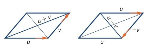
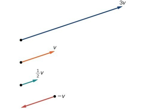
Scalar multiplication stretches or shrinks a vector and can reverse its direction if the scalar is negative.
These geometric operations follow the same algebraic properties found in vector spaces—such as commutativity, associativity, and distributivity — allowing us to interpret abstract vector operations visually as movements and scalings in space.
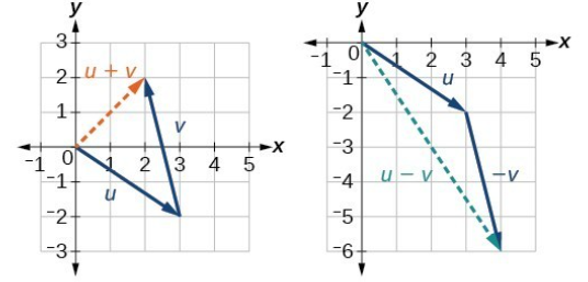
Example 2.9 Let \(\mathbf{u} = [3,-2]\) and \(\mathbf{v} = [-1,4]\). Then \(\mathbf{u} + \mathbf{v}\) and \(\mathbf{u} - \mathbf{v}\) can be computed using vectors: \[\mathbf{u} + \mathbf{v}= [2,2] \;\;\; \text{ and } \;\;\; \mathbf{u} - \mathbf{v} = [4,-6].\]
Exercise 2.3 Both
Exercise 2.4 Show that each of the following are vector spaces:
- \(\mathbb{R}^n\)
- Polynomials
- Continuous functions
- Sequences
Exercise 2.5 Let \(\mathbf{u}, \mathbf{v}, \mathbf{w}\) be vectors, and let \(c, d\) be scalars. Prove each of the following properties:
Commutativity of Addition
\[ \mathbf{u} + \mathbf{v} = \mathbf{v} + \mathbf{u} \]Associativity of Addition
\[ (\mathbf{u} + \mathbf{v}) + \mathbf{w} = \mathbf{u} + (\mathbf{v} + \mathbf{w}) \]Additive Identity
There exists a zero vector \(\mathbf{0}\) such that
\[ \mathbf{v} + \mathbf{0} = \mathbf{v} \]Additive Inverse
For every vector \(\mathbf{v}\), there exists a vector \(-\mathbf{v}\) such that
\[ \mathbf{v} + (-\mathbf{v}) = \mathbf{0} \]Distributive Properties
\[ c(\mathbf{u} + \mathbf{v}) = c\mathbf{u} + c\mathbf{v} \] \[ (c + d)\mathbf{v} = c\mathbf{v} + d\mathbf{v} \]Associativity of Scalar Multiplication
\[ c(d\mathbf{v}) = (cd)\mathbf{v} \]Multiplicative Identity
\[ 1 \mathbf{v} = \mathbf{v} \]
Exercise 2.6 Dot product example
Exercise 2.7