Chapter 3 Continuous Optimization
Machine learning training often involves finding the best set of parameters that minimize an objective function, which measures how well a model fits the data. This search for optimal parameters is formulated as a continuous optimization problem, since the parameters typically take values in \(\mathbb{R}^D\).
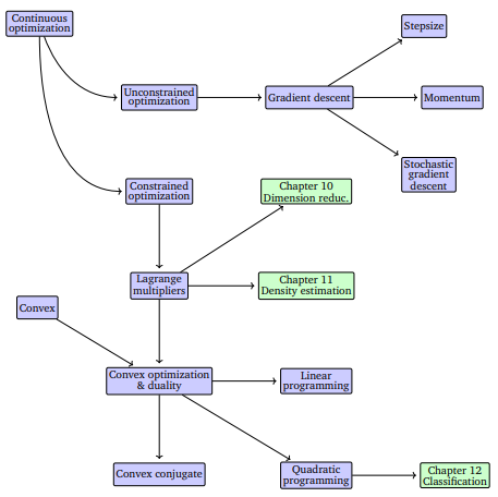
Optimization problems can be divided into two main types:
- Unconstrained optimization, where parameters can take any value in \(\mathbb{R}^D\).
- Constrained optimization, where parameters must satisfy specific restrictions.
Most objective functions in machine learning are differentiable, allowing the use of gradients to find minima. The gradient points in the direction of steepest ascent, so algorithms typically move in the opposite direction (downhill) to minimize the function. The step size determines how far to move along this direction.
The goal is to find points where the gradient is zero — these are stationary points. A stationary point can be:
- A local minimum (second derivative \(> 0\)),
- A local maximum (second derivative \(< 0\)), or
- A saddle point.
An example function
\[
\ell(x) = x^4 + 7x^3 + 5x^2 - 17x + 3
\]
demonstrates multiple stationary points — two minima and one maximum — found by setting the derivative
\[
\frac{d\ell(x)}{dx} = 4x^3 + 21x^2 + 10x - 17 = 0
\]
to zero and analyzing the sign of the second derivative.
In practice, analytical solutions are often not feasible, especially for high-degree polynomials (by the Abel–Ruffini theorem, equations of degree ≥5 cannot be solved algebraically). Instead, we rely on numerical optimization algorithms that iteratively follow the negative gradient.
A key concept introduced later in the chapter is convex optimization. For convex functions, every local minimum is also a global minimum, which guarantees that gradient-based methods will converge to the optimal solution regardless of the starting point. Many machine learning objectives are designed to be convex for this reason.
While the examples here are one-dimensional, the same principles extend to multidimensional optimization, though visualization becomes more challenging. Gradients, step directions, and curvature generalize to higher-dimensional parameter spaces.